


Hypoplastic Sand
Hypoplastic sand is applicable for the modeling of coarse grain soils (sands, gravels). It is a standard phenomenological model, which is the outcome of research at the University of Karlsruhe in the 1990s. The program uses the formulation of the model according to [1]. Similarly to the hypoplastic clay, the model accounts for the nonlinear response of soils both in loading and unloading. In comparison to other models based on the theory of plasticity, it allows for the calculation of total strains only. It thus makes no difference between elastic and plastic strains. The type and location of a potential failure can be represented e.g. by the distribution of the mobilized angle of internal friction.
When describing the soil response, the model allows for reflecting a different stiffness in loading and unloading and the dependence of stiffness and strength on the current mean stress and on the density of soil, which is given by its void ratio. Dense sand dilates in shearing and shows a peak strength followed by softening, loose sand compacts in shearing. After large shear strains both approach the critical state. A single set of parameters thus describes the given sand in all densities and at all stress levels. The critical state surface has in the deviatoric plane the shape of the Matsuoka-Nakai criterion.
Model parameters
The basic variant of the model requires inputting eight material parameters:
- Critical state angle of internal friction φcs
- Granular hardness hs
- Exponent of compression curve n
- Minimum, critical and maximum void ratio at zero pressure ed0, ec0 and ei0
- Pyknotropy exponents α and β
The void ratio of sand lies between three limit values, which decrease with increasing mean stress p:

where ei is the maximum void ratio (the loosest state reached in isotropic compression), ec is the critical void ratio (critical state) and ed is the minimum void ratio (the densest state reached by cyclic shearing with small amplitude). The curve ec(p) represents the compression law of the sand; its shape is given by the parameters hs and n. It must hold ed0 < ec0 < ei0.
Critical state angle of internal friction φcs
- For coarse grain soils it can be estimated from the angle of repose of dry sand
- For finer materials it is determined from a triaxial shear test on a loose sample
- Most common values are in range of 30° - 43°
Granular hardness hs and exponent n
- They determine the shape of the curves of limit void ratios
- They are determined from an oedometric test on a loose sand sample, whose compression curve approximately corresponds to the curve ec(p)
- Both parameters are calibrated together, within the calibrated stress range only their combination matters
- Clean quartz sands calibrated over a wide stress range give hs of the order of 106 kPa and n = 0.25 - 0.4. Silty and clayey sands calibrated at low stresses often give much lower hs (hundreds to thousands of kPa) together with a low n (0.05 - 0.2)
Void ratios ec0, ei0 and ed0
- ec0 is determined from the same oedometric test on loose sand, approximately ec0 ≈ emax (maximum void ratio from the standard index test)
- ei0 can be estimated by the empirical relation ei0 ≈ 1.2 ec0
- ed0 is determined from cyclic shear tests with small amplitude, or it is estimated as ed0 ≈ emin (minimum void ratio from the standard index test) or ed0 ≈ 0.5 ec0
- Most common values are in range of ed0 = 0.35 - 1.05, ec0 = 0.7 - 2.1, ei0 = 0.8 - 2.5
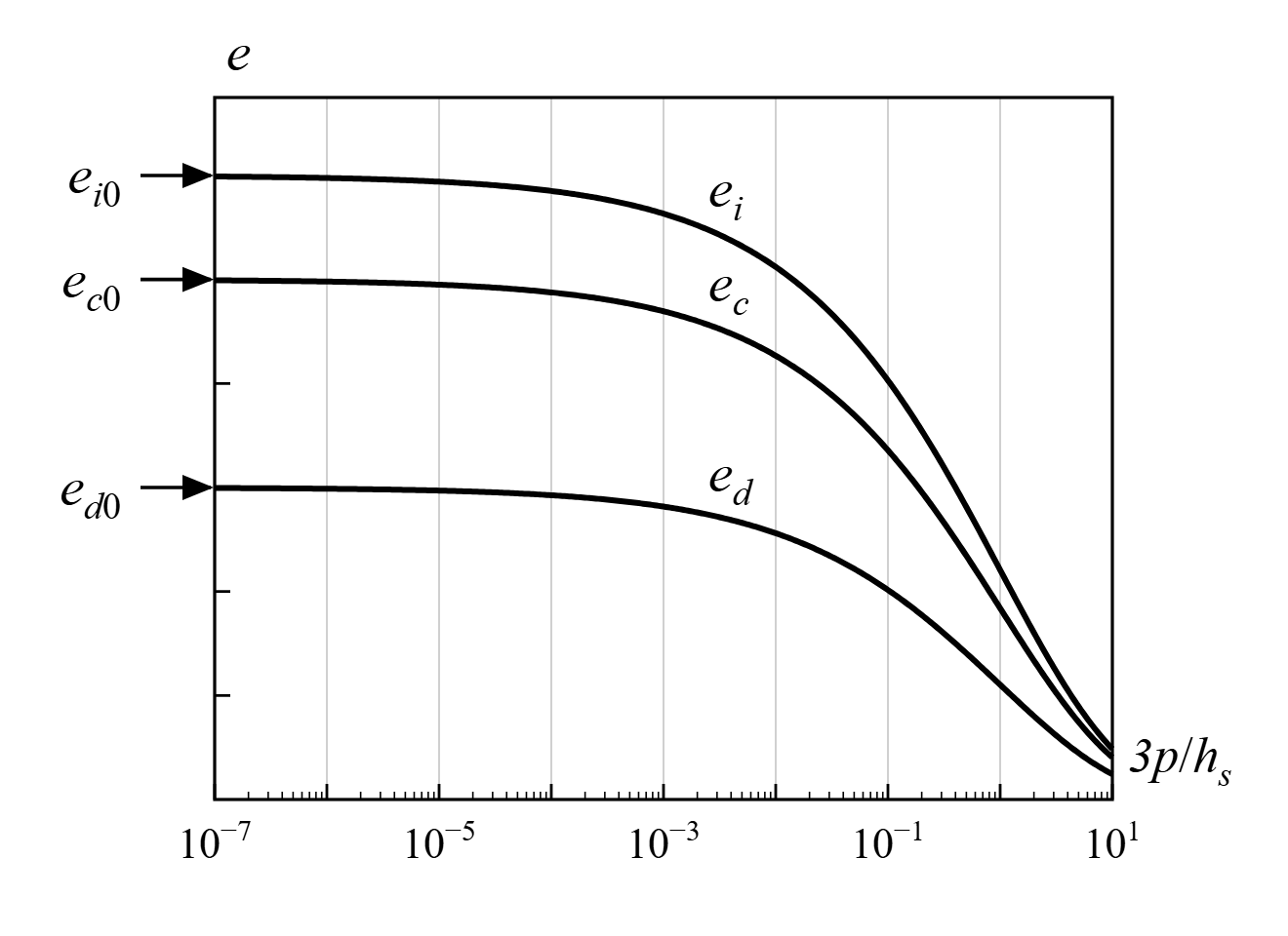 Bounding void ratios depend on mean effective stress.
Pyknotropy exponent α
- It controls the dependence of the peak friction angle on the relative density, increasing α increases the peak friction angle of dense sand
- It is calibrated by simulating a drained triaxial test on a dense sample
- Most common values are in range of 0.03 - 0.5
Pyknotropy exponent β
- It controls the dependence of the stiffness on the relative density, increasing β increases the shear stiffness
- It is calibrated by fitting the stress-strain curve of a drained triaxial test on a dense sample
- Most common values are in range of 1.0 - 6.6
The parameters can be calibrated automatically from laboratory test results with the online tool ExCalibre. Examples of parameters of selected sands [1], [2], [3]:
Soil | φcs [°] | hs [kPa] | n [-] | ed0 [-] | ec0 [-] | ei0 [-] | α [-] | β [-] |
Hochstetten [1] | 33.0 | 1 000 000 | 0.25 | 0.55 | 0.95 | 1.05 | 0.25 | 1.00 |
Karlsruhe [2] | 30.0 | 5 800 000 | 0.28 | 0.53 | 0.84 | 1.00 | 0.13 | 1.05 |
Dobrany [3] | 36.5 | 52 638 | 0.178 | 0.629 | 1.257 | 1.509 | 0.10 | 4.20 |
Kolny [3] | 32.9 | 57 345 | 0.376 | 0.342 | 0.684 | 0.821 | 0.06 | 1.10 |
Kralupy [3] | 36.3 | 1 754 | 0.138 | 0.853 | 1.706 | 2.047 | 0.16 | 2.90 |
Motol [3] | 35.3 | 984 | 0.216 | 0.570 | 1.140 | 1.368 | 0.03 | 2.40 |
Rohatec [3] | 34.3 | 96 157 | 0.353 | 0.388 | 0.776 | 0.931 | 0.12 | 3.80 |
Stvanice [3] | 35.2 | 836 | 0.189 | 0.861 | 1.722 | 2.066 | 0.46 | 4.60 |
Setting initial state of soil
In hypoplastic sand the current state of soil is associated with the current density represented by the void ratio e. Unlike the hypoplastic clay, there is no natural default state for sand, since the same sand may exist at the same stress in any density between ed and ei. The void ratio must therefore always be specified, by exactly one of the following options:
- Initial void ratio ecurr - void ratio of the stressed soil at the current (initial) stress state, it is used as entered
In both cases the void ratio is limited to the range ed ≤ e ≤ ei for the current mean stress. The density of sand can be expressed by the relative density
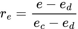
where re = 0 corresponds to the densest state and re = 1 to the critical state. A void ratio close to ed0 thus means dense sand, close to ec0 medium dense to loose sand and close to ei0 very loose sand. Since ec0 ≈ emax and ed0 ≈ emin, for a known relative density ID it is possible to estimate ein ≈ ec0 - ID(ec0 - ed0).
When the task is initialized in the first stage by the K0 procedure, the state of soil is set at the beginning of the following stage from the geostatic stress. In this case it is advisable to specify the initial void ratio ein, which ensures the same relative density at all depths. Sands are usually assumed normally consolidated, i.e. K0 = K0NC = 1 - sin φcs. The overconsolidation ratio OCR and the preoverburden pressure POP are not used by the model, the state of sand is fully described by its void ratio. In addition, the parameter POP would be taken into account in the calculation of the horizontal geostatic stress in the K0 procedure, and therefore it is not recommended to specify it. The effect of previous preloading can be taken into account by a higher value of K0.
Intergranular strain
The basic version of the model is suitable in analyses with a prevailing direction of the stress loading path. In cases with cyclic loading it is more suitable to use an advanced formulation with the concept of intergranular strain [4]. This allows for constraining an unacceptable increase of permanent deformation arising during small repeating changes in load (ratcheting). Introducing intergranular strain allows for the modeling of large stiffness, which soils experience during small strains. The concept of intergranular strain assumes that the total soil deformation consists of a small deformation of an intergranular layer (intergranular strain) and deformation caused by mutual sliding of grains. Changing the load path changes first the intergranular strain. Upon reaching the limit value of the intergranular strain, the deformation associated with the motion of grains sets on.
Adopting the concept of intergranular strain requires five additional parameters:
- Range of elastic intergranular strain R
- Parameters mR and mT control the small strain stiffness
- Parameters βr and χ control the degree of stiffness degradation with increasing strain
These parameters are calibrated after knowing already the material data of the basic hypoplastic model.
Range of elastic intergranular strain R
- It determines the range of maximal intergranular strain
- It is usually considered as material independent constant R = 10-4
Parameters mR and mT
- They determine the multiplier of the very small strain stiffness with respect to the stiffness of the basic model after changing the direction of the strain path by 180° (mR) and by 90° (mT)
- mR is calibrated from the initial shear modulus G0 (e.g. measured by bender elements). Its value cannot be determined directly, it must be found by simulating the test
- If no data are available, mT = 0.4 - 0.7 mR can be assumed
- Most common values of mR are in range of 2 - 8
Parameters βr and χ
- They determine the rate of stiffness degradation with increasing strain
- They can be determined by a parametric study of the stiffness degradation curve or from the cyclic response of soil
- Most common values of parameter βr are in range of 0.1 - 0.5
- Most common values of parameter χ are in range of 1 - 6
For the Hochstetten sand the values R = 10-4, mR = 5.0, mT = 2.0, βr = 0.5 and χ = 6.0 are reported [4].
Notes on the analysis
- The model is available for plane strain and axisymmetric analyses.
- Stresses must be in kPa, consistently with the unit of the parameter hs.
- To avoid problems with zero stress (e.g. at the ground surface), the model is evaluated with the mean stress shifted by pt = 10 kPa. This corresponds to a small apparent cohesion and allows for small tensile stresses.
- The strength of contact elements cannot be derived from the hypoplastic model. Parameters of contacts must be entered separately.
- The tangent stiffness matrix contains only the hypoelastic part of the model. Equilibrium iterations therefore converge more slowly than for elasto-plastic models. If the solution does not converge, it is advisable to reduce the load step.
- The model does not distinguish elastic and plastic strains, results related to plastic strains are therefore not available.
Implementation of the Hypoplastic Clay material model into the GEO5 FEM program is described in detail in the theoretical manual.
Literature:
[1] P.-A. von Wolffersdorff, A hypoplastic relation for granular materials with a predefined limit state surface, Mechanics of Cohesive-Frictional Materials, 1(3):251-271, 1996.
[2] I. Herle, G. Gudehus, Determination of parameters of a hypoplastic constitutive model from properties of grain assemblies, Mechanics of Cohesive-Frictional Materials, 4(5):461-486, 1999.
[3] ExCalibre - soil parameter database, https://soilmodelservice.fsv.cvut.cz/theory/exampleparameters
[4] A. Niemunis, I. Herle, Hypoplastic model for cohesionless soils with elastic strain range, Mechanics of Cohesive-Frictional Materials, 2(4):279-299, 1997.